11 Statistical Functions in R: Common Functions and How They Work
At its core, R programming is a statistical programming language. If you are an R programmer, there’s a good chance you want to make predictions or inferences with data. That’s what we’ll cover in this chapter!
11.1 How Statistical Functions Work in R Programming
A great thing about statistical functions in R is that they often follow the same principles. The steps that apply to one function usually applies to others.
Typically, you’ll use a model function (such as lm()) to create a list object. So long as you assign this object a name, you can apply various other functions to it and evaluate its performance.
The common functions you’ll apply to this model object are:
-
summary(), which summarizes the model parameter estimates and overall model performance -
predict(), which allows you to see what your model predicts on both existing and new data sets -
write_rds(), which allows you to save the model file for future use (requiresreadrpackage) -
anova(), which allows you to generate an analysis of variance on a single model or compare multiple models -
confint(), which allows you to generate the confidence intervals on your model parameters
It’s okay if it’s not clear yet how these concepts work together. I’ll demonstrate them over the next few sections. Keep in mind that even if the model type you want is not covered in this section, these functions apply to most model objects, most of the time.
Towards the end of this chapter, I’ll provide some simple examples that walk you through the common statistical functions and models used in research.
11.2 How to Build a Model in R (Example with Linear Regression)
Let’s say we want to build a model with the mtcars data set. We want a model that uses disp to predict mpg. If you look at the data set below, we can see the summary statistics for those two columns.
##       mpg             disp
##  Min.   :10.40   Min.   : 71.1
##  1st Qu.:15.43   1st Qu.:120.8
##  Median :19.20   Median :196.3
##  Mean   :20.09   Mean   :230.7
##  3rd Qu.:22.80   3rd Qu.:326.0
##  Max.   :33.90   Max.   :472.0
In order to build a model, we’ll use the lm() function. To use this function, we only need to define our formula and our data set:
mod1 <- lm(mpg~disp,data=mtcars)The formula is defined using a ~ sign. This basically implies our regression model is “mpg=disp.”
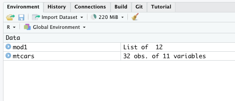
One important thing to note is the type of object this function generates. If you look at the Environment pane, you’ll see this object saved as a list.
This list includes many smaller components that come in handy later. Most other modeling functions in R mimic this workflow as well.
11.3 How to Review Common Model Performance Statistics
Building a model isn’t that hard, as you can tell. Typically though, the real work lays in model evaluation. Most of these summary statistics can be found using the summary() function:
summary(mod1)##
## Call:
## lm(formula = mpg ~ disp, data = mtcars)
##
## Residuals:
## Min 1Q Median 3Q Max
## -4.8922 -2.2022 -0.9631 1.6272 7.2305
##
## Coefficients:
## Estimate Std. Error t value Pr(>|t|)
## (Intercept) 29.599855 1.229720 24.070 < 2e-16 ***
## disp -0.041215 0.004712 -8.747 9.38e-10 ***
## ---
## Signif. codes: 0 '***' 0.001 '**' 0.01 '*' 0.05 '.' 0.1 ' ' 1
##
## Residual standard error: 3.251 on 30 degrees of freedom
## Multiple R-squared: 0.7183, Adjusted R-squared: 0.709
## F-statistic: 76.51 on 1 and 30 DF, p-value: 9.38e-10As you can see, this summary() function reveals a lot about how well this model performs. We can see the adjusted R-square, the F-Statistic, and the individual p-value for the parameter estimate.
You might ask why not just call mod1. Why do we have to use the summary() function? You can do that, but it doesn’t give you nearly the same amount of detail.
mod1##
## Call:
## lm(formula = mpg ~ disp, data = mtcars)
##
## Coefficients:
## (Intercept) disp
## 29.59985 -0.04122The reason will be more clear in a moment. “mod1” is the actual model. While we usually want the summary() output after building the model, there are several other things we want to evaluate. If the output of the lm() function didn’t produce a model, but a summary like we saw, it would be more difficult to apply other functions, such as predict() and confint(), to it.
Also, summary() is a universal function within R. It can also be applied to data frames and vectors. Not just the lm() output.
11.3.1 It’s Useful to Save the Summary Output
Sometimes, you may want to evaluate one model against another. Whenever that happens, it’s useful to create another object for the summary output of the model. This will allow you to select individual pieces of the output you saw above.
For example, I can create a new list for model 1’s summary. I can then use the $ notation to call individual performance indicators for that model, such as adj.r.squared or the fstatistic.
  mod1_summary <- summary(mod1)
  mod1_summary$adj.r.squared
  mod1_summary$fstatistic
You can determine what values are available in a model summary using the names() function:
names(mod1_summary)## [1] "call" "terms" "residuals" "coefficients"
## [5] "aliased" "sigma" "df" "r.squared"
## [9] "adj.r.squared" "fstatistic" "cov.unscaled"11.4 How to Make Predictions with a Model
Many researchers are more interested in the “inferential” side of statistics. In plain English, you’re hoping to prove or disprove a relationship between one variable and another. Others time, you may want to use your model to predict future events or outcomes. This is more common for data scientists like me.
You can use the predict() function to make predictions on new data. Actually, you can use this function without new data simply by plugging the model object name in. This will show you what the model predicts using the original data set (which is often a useful model performance indicator on its own).
predict(mod1)## Mazda RX4 Mazda RX4 Wag Datsun 710 Hornet 4 Drive
## 23.00544 23.00544 25.14862 18.96635
## Hornet Sportabout Valiant Duster 360 Merc 240D
## 14.76241 20.32645 14.76241 23.55360
## Merc 230 Merc 280 Merc 280C Merc 450SE
## 23.79677 22.69220 22.69220 18.23272
## Merc 450SL Merc 450SLC Cadillac Fleetwood Lincoln Continental
## 18.23272 18.23272 10.14632 10.64090
## Chrysler Imperial Fiat 128 Honda Civic Toyota Corolla
## 11.46520 26.35622 26.47987 26.66946
## Toyota Corona Dodge Challenger AMC Javelin Camaro Z28
## 24.64992 16.49345 17.07046 15.17456
## Pontiac Firebird Fiat X1-9 Porsche 914-2 Lotus Europa
## 13.11381 26.34386 24.64168 25.68030
## Ford Pantera L Ferrari Dino Maserati Bora Volvo 142E
## 15.13335 23.62366 17.19410 24.61283Let’s say we have new values for disp. We want to see what our model predicts for mpg using these new records. All we have to do is specify the model object name and the data set object name in the predict() function:
  disp_new <- data.frame(disp=c(rnorm(15,240,30))) #this simply generates random numbers
  predict(mod1,disp_new)
## 1 2 3 4 5 6 7 8
## 21.92072 19.57914 19.62402 18.37712 20.86951 18.68507 20.79849 19.15828
## 9 10 11 12 13 14 15
## 17.89549 20.64230 20.99769 17.17329 21.15449 18.20183 19.61650As you can imagine, this predict() function comes in handy. And it’s a common feature for most model objects produced in other R packages. I’ve used this for neural nets and other more advanced predictive algorithms. It comes up again and again.
11.5 How to Save Your Model to Use Later
It’s quite common to share models between colleagues. Maybe another researcher wants to re-produce what you created or another data scientist will integrate your model into a Shiny app.
That’s where .rds files come in handy.
.rds files allow you to save objects on your desktop or user directory for later use.
You’ll need to load the readr package to create these file types. After that, you’ll use the write_rds() function to create an .rds file and read_rds() to load it. (You may need to install this package using install.packages().)
After running the previous script, you’ll see an .rds file appear in your current working directory (usually your project directory or your default user directory). You can specify the file path in that script above between the two quotations marks.

If you want to re-use this model, you can simply reload the .rds file using the read_rds() function. Be sure to assign this object a name to make it work.
model_reload <- read_rds("mod1.rds")And here’s the cool part about this .rds file - you don’t need to reload the original data set to make this new model work! If you feed it new data, it’ll make new predictions. This comes in handy whenever you build Shiny apps or want to “productionalize” the model.
  disp_new <- data.frame(disp=c(rnorm(15,240,30)))
  predict(model_reload,disp_new)
## 1 2 3 4 5 6 7 8
## 20.82545 21.27865 20.16891 19.18273 18.64478 19.26571 19.85724 21.91752
## 9 10 11 12 13 14 15
## 17.48599 19.03953 20.60156 20.60352 18.19875 20.04392 20.7724111.6 How to Add Multiple Parameters to a Model
You can add additional parameters to your model by adding to the formula in the lm() function. Let’s say we want to add the drat and wt variables to your regression model. All you have to do specify both variables with a + sign between them.
##
## Call:
## lm(formula = mpg ~ disp + drat + wt, data = mtcars)
##
## Residuals:
##     Min      1Q  Median      3Q     Max
## -3.2342 -2.3719 -0.3148  1.6315  6.2820
##
## Coefficients:
##              Estimate Std. Error t value Pr(>|t|)
## (Intercept) 31.043257   7.099792   4.372 0.000154 ***
## disp        -0.016389   0.009578  -1.711 0.098127 .
## drat         0.843965   1.455051   0.580 0.566537
## wt          -3.172482   1.217157  -2.606 0.014495 *
## ---
## Signif. codes:  0 '***' 0.001 '**' 0.01 '*' 0.05 '.' 0.1 ' ' 1
##
## Residual standard error: 2.951 on 28 degrees of freedom
## Multiple R-squared:  0.7835, Adjusted R-squared:  0.7603
## F-statistic: 33.78 on 3 and 28 DF,  p-value: 1.92e-09
As you can see above, those variables aren’t necessarily the best addition or combination. But since it’s an example, we won’t worry too much about it here.
11.7 How to Add a Categorical Variable to a Model
So far, I’ve only shown you how to add continuous variables. What if we want to add a categorical variable?
If a column in a data frame has character values (i.e., text), a model function will automatically treat it as a categorical variable. If it contains numeric values, we’ll need to make it a factor. (Review our chapter on object-types for a quick refresher on this topic.)
##
## Call:
## lm(formula = mpg ~ disp + factor(cyl), data = mtcars)
##
## Residuals:
##     Min      1Q  Median      3Q     Max
## -4.8304 -1.5873 -0.5851  0.9753  6.3069
##
## Coefficients:
##              Estimate Std. Error t value Pr(>|t|)
## (Intercept)  29.53477    1.42662  20.703  < 2e-16 ***
## disp         -0.02731    0.01061  -2.574  0.01564 *
## factor(cyl)6 -4.78585    1.64982  -2.901  0.00717 **
## factor(cyl)8 -4.79209    2.88682  -1.660  0.10808
## ---
## Signif. codes:  0 '***' 0.001 '**' 0.01 '*' 0.05 '.' 0.1 ' ' 1
##
## Residual standard error: 2.95 on 28 degrees of freedom
## Multiple R-squared:  0.7837, Adjusted R-squared:  0.7605
## F-statistic: 33.81 on 3 and 28 DF,  p-value: 1.906e-09
11.8 How to Add Transformed Variables to a Model
Quite often, you may need to transform your variables to make them work in a model. Let’s say you want to build a log-log model. That has different meanings depending on your field of study, but in econometrics, a log-log model transforms both the inputs and the outputs using the natural logarithm. (This is how they often calculate price elasticity.)
You could simply do these transformations in the formula argument in the lm() function. If you look below, I simply wrap both the independent and dependent variable with the log() function:
##
## Call:
## lm(formula = log(mpg) ~ log(disp), data = mtcars)
##
## Residuals:
##      Min       1Q   Median       3Q      Max
## -0.22758 -0.08874 -0.00791  0.07970  0.32143
##
## Coefficients:
##             Estimate Std. Error t value Pr(>|t|)
## (Intercept)  5.38097    0.20803   25.87  < 2e-16 ***
## log(disp)   -0.45857    0.03913  -11.72 1.01e-12 ***
## ---
## Signif. codes:  0 '***' 0.001 '**' 0.01 '*' 0.05 '.' 0.1 ' ' 1
##
## Residual standard error: 0.1282 on 30 degrees of freedom
## Multiple R-squared:  0.8207, Adjusted R-squared:  0.8148
## F-statistic: 137.3 on 1 and 30 DF,  p-value: 1.006e-12
This works okay for smaller models. If you want to transform several variables, it’s usually easier to create new ones in the data set prior to building the model:
  cars_log <- mtcars
  cars_log$mpg_log <- log(cars_log$mpg)
  cars_log$disp_log <- log(cars_log$disp)
  cars_log$qsec_log <- log(cars_log$qsec)

  summary(cars_log[c(1,3,7,12,13,14)])
## mpg disp qsec mpg_log
## Min. :10.40 Min. : 71.1 Min. :14.50 Min. :2.342
## 1st Qu.:15.43 1st Qu.:120.8 1st Qu.:16.89 1st Qu.:2.736
## Median :19.20 Median :196.3 Median :17.71 Median :2.955
## Mean :20.09 Mean :230.7 Mean :17.85 Mean :2.958
## 3rd Qu.:22.80 3rd Qu.:326.0 3rd Qu.:18.90 3rd Qu.:3.127
## Max. :33.90 Max. :472.0 Max. :22.90 Max. :3.523
## disp_log qsec_log
## Min. :4.264 Min. :2.674
## 1st Qu.:4.794 1st Qu.:2.827
## Median :5.269 Median :2.874
## Mean :5.285 Mean :2.877
## 3rd Qu.:5.786 3rd Qu.:2.939
## Max. :6.157 Max. :3.131We can then use those new columns in the model function:
##
## Call:
## lm(formula = mpg_log ~ disp_log + qsec_log, data = cars_log)
##
## Residuals:
##      Min       1Q   Median       3Q      Max
## -0.22998 -0.08890 -0.00661  0.08202  0.32098
##
## Coefficients:
##             Estimate Std. Error t value Pr(>|t|)
## (Intercept)  5.26474    0.88872   5.924 1.96e-06 ***
## disp_log    -0.45587    0.04454 -10.234 3.89e-11 ***
## qsec_log     0.03544    0.26323   0.135    0.894
## ---
## Signif. codes:  0 '***' 0.001 '**' 0.01 '*' 0.05 '.' 0.1 ' ' 1
##
## Residual standard error: 0.1303 on 29 degrees of freedom
## Multiple R-squared:  0.8208, Adjusted R-squared:  0.8085
## F-statistic: 66.43 on 2 and 29 DF,  p-value: 1.486e-11
11.9 How to Add Variable Interactions to a Model
It’s not uncommon to include interactions in your model, especially if you have two variables that seem to be correlated. To create these interactions, you simply use the * between them in the model formula.
##
## Call:
## lm(formula = mpg ~ drat + wt + drat * wt, data = mtcars)
##
## Residuals:
##     Min      1Q  Median      3Q     Max
## -3.8913 -1.8634 -0.3398  1.3247  6.4730
##
## Coefficients:
##             Estimate Std. Error t value Pr(>|t|)
## (Intercept)    5.550     12.631   0.439   0.6637
## drat           8.494      3.321   2.557   0.0162 *
## wt             3.884      3.798   1.023   0.3153
## drat:wt       -2.543      1.093  -2.327   0.0274 *
## ---
## Signif. codes:  0 '***' 0.001 '**' 0.01 '*' 0.05 '.' 0.1 ' ' 1
##
## Residual standard error: 2.839 on 28 degrees of freedom
## Multiple R-squared:  0.7996, Adjusted R-squared:  0.7782
## F-statistic: 37.25 on 3 and 28 DF,  p-value: 6.567e-10
You actually don’t even need to specify the variables individually. For example, rather than mpg~drat+wt+drat*wt, you can simply use mpg~drat*wt and the function will treat them individually and as interactions.
##
## Call:
## lm(formula = mpg ~ drat * wt, data = mtcars)
##
## Residuals:
##     Min      1Q  Median      3Q     Max
## -3.8913 -1.8634 -0.3398  1.3247  6.4730
##
## Coefficients:
##             Estimate Std. Error t value Pr(>|t|)
## (Intercept)    5.550     12.631   0.439   0.6637
## drat           8.494      3.321   2.557   0.0162 *
## wt             3.884      3.798   1.023   0.3153
## drat:wt       -2.543      1.093  -2.327   0.0274 *
## ---
## Signif. codes:  0 '***' 0.001 '**' 0.01 '*' 0.05 '.' 0.1 ' ' 1
##
## Residual standard error: 2.839 on 28 degrees of freedom
## Multiple R-squared:  0.7996, Adjusted R-squared:  0.7782
## F-statistic: 37.25 on 3 and 28 DF,  p-value: 6.567e-10
11.10 How to Calculate Model Confidence Intervals
Even though the p-value tells you whether the variable is statistically significant, it’s often a best practice to include confidence intervals in your analysis. R makes this very easy! Simply wrap the confint() function around your model object.
confint(mod2)## 2.5 % 97.5 %
## (Intercept) 16.49999311 45.586521444
## disp -0.03600944 0.003231128
## drat -2.13657099 3.824501624
## wt -5.66571478 -0.679250218If you want to have a different critical value, you can change it using the level argument.
confint(mod2,level=.9)## 5 % 95 %
## (Intercept) 18.96558187 4.312093e+01
## disp -0.03268312 -9.519212e-05
## drat -1.63126649 3.319197e+00
## wt -5.24302525 -1.101940e+00See ?confint to read more about the function.
11.11 How to Calculate Analysis of Variance Between Models
You’ll often need to compare models with more parameter estimates to simpler ones. To do so, you simply create your two models and then use the anova() function:
anova(mod1,mod2)## Analysis of Variance Table
##
## Model 1: mpg ~ disp
## Model 2: mpg ~ disp + drat + wt
## Res.Df RSS Df Sum of Sq F Pr(>F)
## 1 30 317.16
## 2 28 243.75 2 73.405 4.216 0.02509 *
## ---
## Signif. codes: 0 '***' 0.001 '**' 0.01 '*' 0.05 '.' 0.1 ' ' 111.12 Other Common Model Types - Logistic Regression
Chances are, you want to do more than a linear regression. Most statistics or ML textbooks will cover the programming steps involved for a particular model type. Those models usually follow the same procedures I highlighted earlier.
That said though, I can provide some general functions used in the more common statistical models, such as logistic regression and anova models.
To run a logistic model, you can use the glm() function. In the script below, I build use mpg and wt to predict whether vs is a 1 or a 0. I use the family argument to make it a logistic model.
##
## Call:
## glm(formula = vs ~ mpg + wt, family = binomial(link = "logit"),
##     data = mtcars)
##
## Deviance Residuals:
##     Min       1Q   Median       3Q      Max
## -2.2020  -0.5835  -0.2311   0.5376   1.7142
##
## Coefficients:
##             Estimate Std. Error z value Pr(>|z|)
## (Intercept) -12.5412     8.4660  -1.481   0.1385
## mpg           0.5241     0.2604   2.012   0.0442 *
## wt            0.5829     1.1845   0.492   0.6227
## ---
## Signif. codes:  0 '***' 0.001 '**' 0.01 '*' 0.05 '.' 0.1 ' ' 1
##
## (Dispersion parameter for binomial family taken to be 1)
##
##     Null deviance: 43.860  on 31  degrees of freedom
## Residual deviance: 25.298  on 29  degrees of freedom
## AIC: 31.298
##
## Number of Fisher Scoring iterations: 6
The glm() function has a larger range of model types than the lm() function. I suggest reviewing it with ?glm in the console whenever you want to build a particular type of linear model not yet discussed here. The family argument may provide the right model type you need.
Just like we did for the linear regression model, we can use the confint() functions on this model object to generate a confidence interval. You can see this below:
confint(mod7)## Waiting for profiling to be done...## 2.5 % 97.5 %
## (Intercept) -31.90842474 2.921046
## mpg 0.09326514 1.165436
## wt -1.91815266 2.936813You can also use the predict() function on this model.
11.13 Other Common Model Types - Anova Models
To build an ANOVA model, you’ll use the aov() function. This function follows a similar process to the lm() function and actually generates a regression model using the formula you enter.
As you’ll learn in your stats class, many ANOVA models focus on categorical variables to determine whether there’s a difference in the mean outcome. A common model for this scenario is a fixed-effects model.
Let’s convert a few of our cars data into factors, so that we can build a fixed-effects model.
  mtcars_factor <- mtcars
  mtcars_factor$gear <- factor(mtcars_factor$gear)
  mtcars_factor$vs <- factor(mtcars_factor$vs)
Remember, most model functions in R will treat numeric inputs as a continuous variable. Since we want to treat these variables (which range includes the labels 0, 1, 3, and 4), we need to ensure that the function we run treats them as categorical. That’s why we factor them.
Now we can build the fixed-effects model using the aov() function:
##             Df Sum Sq Mean Sq F value   Pr(>F)
## vs           1  496.5   496.5  29.407 8.74e-06 ***
## gear         2  156.8    78.4   4.642   0.0182 *
## Residuals   28  472.8    16.9
## ---
## Signif. codes:  0 '***' 0.001 '**' 0.01 '*' 0.05 '.' 0.1 ' ' 1
The summary() function also gives you the ANOVA table for this model and allows you to determine which group explains the most variation.
Sometimes you still want a model that shows you the actual impact a variable has on the expected output. We can do this by first running the lm() function with our formula.
##
## Call:
## lm(formula = mpg ~ vs + gear, data = mtcars_factor)
##
## Residuals:
##     Min      1Q  Median      3Q     Max
## -7.7185 -2.7227  0.2755  1.9300  8.3815
##
## Coefficients:
##             Estimate Std. Error t value Pr(>|t|)
## (Intercept)   14.924      1.124  13.273 1.33e-13 ***
## vs1            5.911      1.863   3.173  0.00364 **
## gear4          4.683      1.981   2.364  0.02525 *
## gear5          5.273      2.122   2.485  0.01919 *
## ---
## Signif. codes:  0 '***' 0.001 '**' 0.01 '*' 0.05 '.' 0.1 ' ' 1
##
## Residual standard error: 4.109 on 28 degrees of freedom
## Multiple R-squared:  0.5802, Adjusted R-squared:  0.5352
## F-statistic:  12.9 on 3 and 28 DF,  p-value: 1.787e-05
And you can reference the model object again in the same aov() function from earlier and get your ANOVA table.
summary(mod8)## Df Sum Sq Mean Sq F value Pr(>F)
## vs 1 496.5 496.5 29.407 8.74e-06 ***
## gear 2 156.8 78.4 4.642 0.0182 *
## Residuals 28 472.8 16.9
## ---
## Signif. codes: 0 '***' 0.001 '**' 0.01 '*' 0.05 '.' 0.1 ' ' 1## Df Sum Sq Mean Sq F value Pr(>F)
## vs 1 496.5 496.5 29.407 8.74e-06 ***
## gear 2 156.8 78.4 4.642 0.0182 *
## Residuals 28 472.8 16.9
## ---
## Signif. codes: 0 '***' 0.001 '**' 0.01 '*' 0.05 '.' 0.1 ' ' 111.14 Things to Remember
- Building and evaluating models often follows the same steps, regardless of the functions you use
- The model function (
lm(),glm(),aov(), etc.) produces a list - You can assign that list a name and reference it again
- You can get most model performance metrics with the
summary()function - You can use that model object to make predictions on both new and existing data with the
predict()function - You can use that model object to generate confidence intervals with the
confint()function - You evaluate two models against one another with the
anova()function - You can export your model (without exporting the data) using the
write_rds()function
11.15 Exercises
- Using the data set iris (
data(iris)), build a linear regression model that uses Sepal.Length and Sepal.Width to predict Petal.Length. Assign the model the name “PracticeModel.” - Determine whether the two parameters are statistically significant. (i.e., their p-values are less than 0.05.)
- Predict the value of Petal.Length with a Sepal.Length of 5 and a Sepal.Width of 3.25. (Hint: create a single row data frame with those two values assigned to their respective column names.)
- Determine the model’s confidence intervals.